DeepSeek’s mHC Paper, Explained for the Rest of Us
Of all the AI labs right now, DeepSeek is the one I find most interesting. The big US labs’ dominant lever has been scale (compute, data, and infrastructure), and they do plenty of algorithmic work too. But DeepSeek has been unusually willing to revisit plumbing-layer assumptions that others treat as done, and that’s what makes their papers so fun to read.
GRPO is a good example. PPO-style RLHF typically trains a separate critic/value network to compute advantages, which adds an extra model to train and run during updates (more memory, more compute, more optimization instability). DeepSeek’s GRPO drops the critic: sample several completions, score them, and use the group mean as the baseline. In their setup it stayed competitive while cutting overhead by removing the value network entirely. That’s the kind of thing they do.
Now they’ve gone after the skip-connection topology that every major architecture relies on. Their paper mHC: Manifold-Constrained Hyper-Connections rethinks how information flows between layers during training.
The paper is pretty math-heavy. (I won’t pretend the notation didn’t take me a few passes.) But the core idea is straightforward once you get past it. And the key mechanism involves an algorithm from 1967.
A Quick Refresher: Backpropagation and the Gradient Problem
If you’ve taken a machine learning course, you know the basic loop. You have a neural network with layers. Each layer transforms the input, passes it to the next. At the end, you compare the output to what you wanted, compute a loss, and use gradient descent to update the weights.
The “gradient” part is where it gets tricky. To update the weights in, say, layer 3 of a 5-layer network, you need the sensitivity of the loss to $W_3$: how much changing $W_3$ would change the loss. That means working backwards from the output using the chain rule, multiplying the local sensitivities at each step. That’s backpropagation, and concretely it looks like this:
\[\frac{\partial \mathcal{L}}{\partial W_3} = \frac{\partial \mathcal{L}}{\partial x_5} \cdot \frac{\partial x_5}{\partial x_4} \cdot \frac{\partial x_4}{\partial x_3} \cdot \frac{\partial x_3}{\partial W_3}\]That’s four multiplicative factors just for layer 3 in a 5-layer network. (Formally these are Jacobians, i.e. matrices of partial derivatives, so the chain rule is really a chain of matrix multiplications. But the scalar intuition holds: multiply a bunch of local sensitivities together.) And this product can become numerically unstable in deep nets, shrinking to near-zero or blowing up entirely. In general, for a network with $N$ layers, the gradient at layer $l$ looks like:
\[\frac{\partial \mathcal{L}}{\partial W_l} = \frac{\partial \mathcal{L}}{\partial x_N} \cdot \frac{\partial x_N}{\partial x_{N-1}} \cdot \frac{\partial x_{N-1}}{\partial x_{N-2}} \cdots \frac{\partial x_{l+1}}{\partial x_l} \cdot \frac{\partial x_l}{\partial W_l}\]You’re multiplying a long chain of local derivatives together. If the typical gain of those derivatives is a bit less than 1, the signal shrinks exponentially as you go deeper. The early layers barely learn because the gradient has decayed by the time it reaches them. And if the gain is a bit more than 1, the opposite happens: it blows up and training goes off the rails.
People call these vanishing and exploding gradients, and for a long time they were a key reason training very deep networks was brittle.
ResNet: The Fix That Worked (Mostly)
In 2015, He et al. proposed a deceptively simple idea: instead of asking each layer to learn a whole new transformation, let it learn a correction to its input, and always keep a clean shortcut path that carries information forward unchanged. These are residual (or skip) connections.
\[x_{l+1} = x_l + F_l(x_l)\]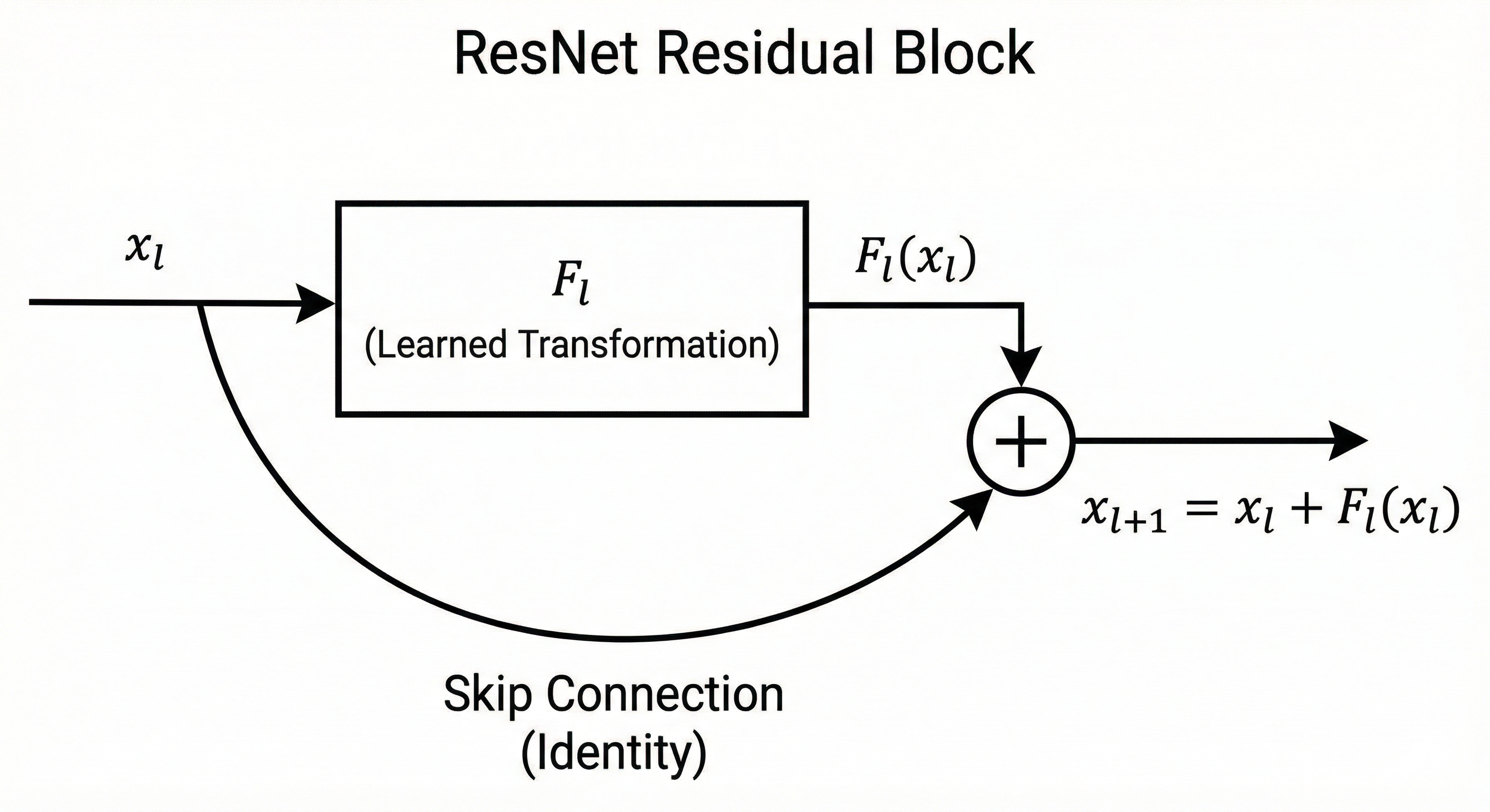
The $x_l$ term is the skip connection. The layer only needs to learn $F_l(x_l)$: the correction. Embarrassingly simple, but it changed everything.
The intuition is that skip connections make “do nothing” the default. If a block isn’t sure what to do yet (especially early in training), it can keep $F_l(x_l) \approx 0$ and just pass $x_l$ through. A deep network no longer has to learn a fragile sequence of transformations just to preserve information. It can start as something close to an identity mapping, then gradually learn a stack of small improvements.
Why does this help with gradients? When you differentiate, that shortcut path shows up as a direct pass-through:
\[\frac{\partial x_{l+1}}{\partial x_l} = I + \frac{\partial F_l}{\partial x_l}\]Notice the $I$ (identity matrix). It represents the direct path that carries the signal forward. So even if the learned part $\frac{\partial F_l}{\partial x_l}$ is small or noisy, there’s still a stable route for gradients to flow through.
It’s tempting to summarize this as “you add 1 to the gradient,” but that’s not quite right. These are matrices, not scalars, and gradients can still shrink or grow. The real point is that the learning signal is no longer forced to pass through only the learned transform at every layer. There’s always a clean baseline route, which makes it much harder for the gradient to get completely strangled just because the network is deep.
This was a breakthrough. ResNet reached 152 layers and won ImageNet 2015. Before that, the deepest winners were VGG at 19 layers and GoogLeNet at 22. Every major architecture since then uses the same pattern. Transformers do it too: each sub-layer proposes an update, and the model adds it back into an ongoing residual stream.
But there’s still a catch. If you expand the recursion across many layers:
\[x_N = x_0 + \sum_{l=0}^{N-1} F_l(x_l)\]What this is really saying: a residual network maintains a single persistent state vector $x$ (the residual stream), and every layer adds its update into that same stream. Each layer has plenty of internal activations (attention heads, MLP hidden states, etc.), but those are temporary. The residual stream is the one thing that survives across depth. Every block reads from it, computes an update, and writes back into it.
Think of $x_0$ as a shared document being passed down a hallway of 200 people, where each person’s edit is one of those $F_l$ terms in the sum. The skip connection guarantees the original document doesn’t get lost. But if too many people edit the same paragraphs for different reasons, the document gets harder to keep coherent. Later editors spend time cleaning up earlier edits instead of making progress. In practice you see this as “add-then-cancel” behavior: one layer writes a feature, a later layer partially undoes it, another rewrites it in a different form. The model can still learn, but it’s working harder than it should.
For most practical networks, this tradeoff is fine. But at the frontier, when you’re training very deep models aggressively, the details of how updates get mixed into that shared stream start to matter.
Hyper-Connections: A Good Idea with a Stability Problem
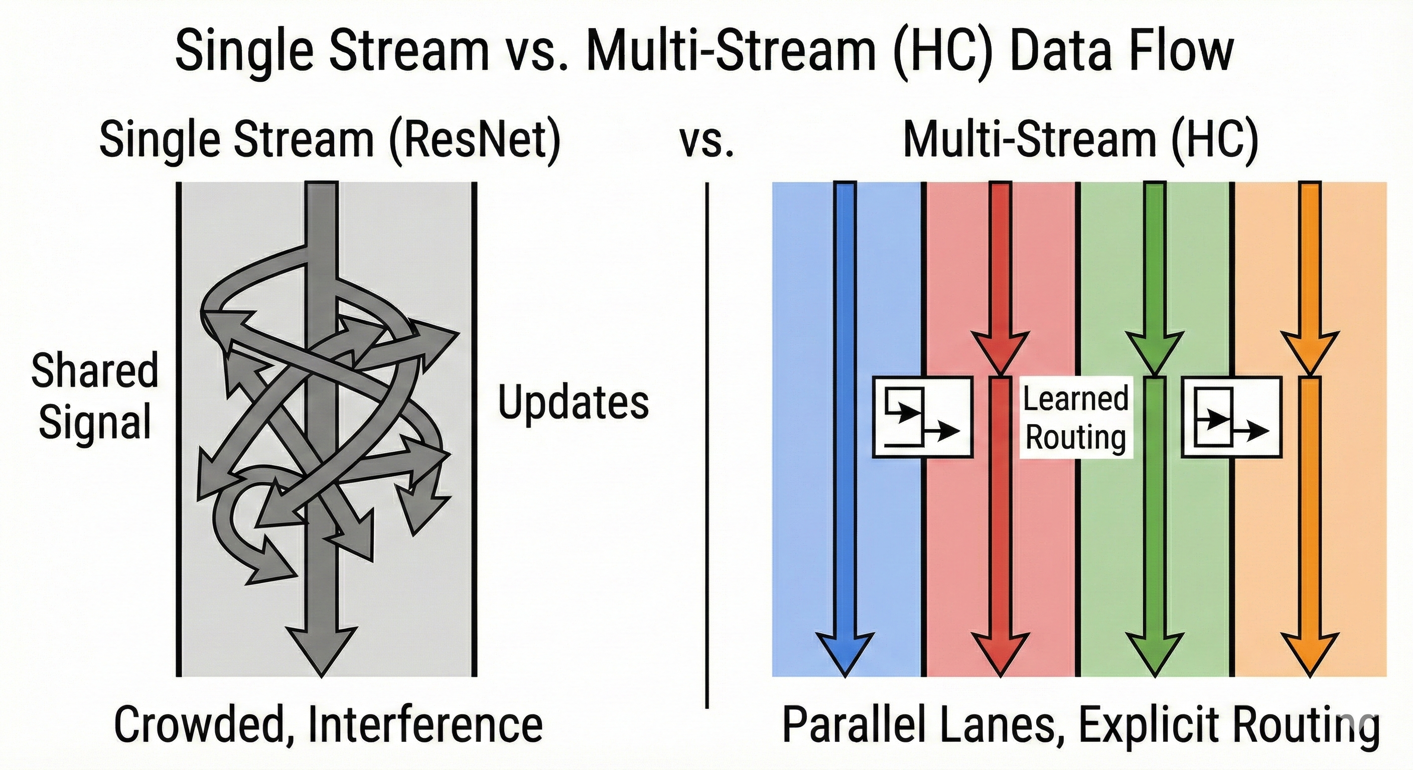
So we have a real limitation: one shared stream where everything has to coexist, and as depth grows, things interfere. A natural question is: what if we gave the network more than one long-lived stream, so information doesn’t all have to share the same lane?
That’s what Hyper-Connections (HC) do. Originally proposed by ByteDance and published at ICLR 2025, HC replaces the single residual stream with $n$ parallel streams (typically $n = 4$), then lets each layer learn where to read from and where to write to.1
Here $H_l^{res}$ is an $n \times n$ matrix controlling how the streams mix on the skip path, $H_l^{pre}$ selects which streams feed into the layer, and $H_l^{post}$ routes the output back.
Why does this help? Think back to our shared-document analogy. With one stream, if you want to preserve two different kinds of information across depth (say, structural scaffolding vs. content), they have to coexist in the same vector, and every layer keeps rewriting it. With $n$ lanes, the model gets separate parking spaces. Some lanes can become stable carriers, others can be scratch space for fast-changing features, and layers can preferentially read from or write to whichever lane they need. Remember the “add-then-cancel” problem? Multiple lanes give the system more ways to avoid it, because updates can land in less-crowded substreams instead of all piling into the same place. A layer can even learn something like “store this in lane 3” and trust that later layers will know to read lane 3 when they need it. That’s explicit routing across depth, rather than hoping a feature survives hundreds of layers of implicit mixing.
But remember why ResNet was stable: the skip path was literally “copy the input forward.” That gave you a safe fallback. HC replaces that safe copy with a learned mixing on the skip path (the $H_l^{res}$ term). And when you stack many layers, those learned mixes multiply across depth:
\[x_N = \Big(H_{N-1}^{res} H_{N-2}^{res} \cdots H_0^{res}\Big) x_0 + \ldots\]where the remaining terms are the per-layer updates, each multiplied by the residual-mixing matrices above it. The important thing is that ordered product on the left. Unlike ResNet’s identity skip path, HC’s skip path is a product of learned matrices, so its gain can drift far from 1. And nothing in the formulation stops it from amplifying signals wildly. In practice, DeepSeek measured the gain of this composite mapping and found it spiking to around 3,000x in some layers. The ideal would be close to 1. At 3,000x, training is unreliable. DeepSeek observed sudden loss spikes and unstable gradient norms, and at larger scales the whole thing can fall apart entirely.
ResNet gives you a stable pass-through, but everything shares one stream. HC gives you multiple streams and learned routing, but the skip path is no longer safe by default. More expressivity, less stability.
mHC: Constraining the Chaos
mHC’s key idea: keep HC’s routing flexibility, but constrain the skip-path mixing so it can’t run away.
The tool they reach for is a doubly stochastic matrix. Sounds intimidating, but it’s one of the simplest ideas in linear algebra. (The name is doing all the heavy lifting here.) A matrix is doubly stochastic if:
- Every entry is non-negative
- Every row sums to 1
- Every column sums to 1
Think of it as a “mixing” matrix: each output lane is a weighted average of the input lanes. It redistributes weight across streams instead of letting the skip path arbitrarily rescale them.
Back to HC’s stability problem. The issue was that stacking many layers of learned $H_l^{res}$ mixing could turn the skip path into a huge amplifier. If each $H_l^{res}$ is doubly stochastic, its row sums and column sums are fixed at 1, which directly controls the gain metric the paper tracks. And because the product of doubly stochastic matrices is also doubly stochastic, stacking hundreds of layers keeps those gains pinned near 1.
That’s the constraint in the paper’s title. They force each $H_l^{res}$ to be (approximately) doubly stochastic.2 The streams can still mix and reroute in complex ways, but the mixing can never become an amplifier.
In practice, the gain that was spiking to 3,000x with unconstrained HC drops to about 1.6x with mHC.3 In the paper’s experiments, that was enough to eliminate the loss spikes, keep gradient norms stable, and hold the performance advantage as they scaled from 3B to 27B parameters.
The 1967 Algorithm That Makes It Work
So you need each layer’s $H_l^{res}$ (the $n \times n$ matrix that mixes the streams on the skip path) to be doubly stochastic. How do you enforce that during training?
You could try to parameterize the matrix directly, but that’s awkward. Doubly stochastic matrices form a complicated constraint set, and your optimizer (Adam, SGD, whatever) doesn’t know about it. It just updates parameters with gradients and hopes for the best.
The trick mHC uses is the Sinkhorn-Knopp algorithm, published by Richard Sinkhorn in 1967. The idea: let the optimizer update $\tilde{H}_l^{res}$ freely (no constraints), then after each update, project it to a doubly stochastic $H_l^{res}$ via Sinkhorn-Knopp. Concretely:
- Take $\tilde{H}_l^{res}$ as the optimizer left it (an $n \times n$ matrix of unconstrained real numbers)
- Exponentiate every entry so they’re all positive
- Normalize each row (divide by row sum)
- Normalize each column (divide by column sum)
- Repeat steps 3-4
Seriously, that’s the whole algorithm. Here it is in Python:
import numpy as np

def sinkhorn_knopp(M, iterations=20):
    M = M - M.max()            # stability: prevent exp overflow
    M = np.exp(M)              # make all entries positive
    for _ in range(iterations):
        M = M / M.sum(axis=1, keepdims=True)  # normalize rows
        M = M / M.sum(axis=0, keepdims=True)  # normalize columns
    return M
That’s the core idea in seven lines. I stared at the paper’s formal notation for a while before realizing it was just this. (A production implementation would add numerical stability tricks like log-space computation and epsilon guards, but the algorithm is the same.) Sinkhorn proved in 1967 that this process converges to a doubly stochastic matrix (given a positive starting matrix, which the exponentiation guarantees). The proof involves some nice properties of positive matrices, but the algorithm itself is about as simple as it gets.
In mHC, the actual procedure is:
\[M^{(0)} = \exp(\tilde{H}_l^{res})\] \[M^{(t)} = T_c(T_r(M^{(t-1)}))\]where $T_r$ normalizes rows and $T_c$ normalizes columns (matching the order in the code above). They run 20 iterations, which is enough for a close approximation at low overhead.
The $\exp$ at the start ensures all entries are positive (you can’t have a doubly stochastic matrix with negative entries). Then Sinkhorn-Knopp does the rest. The underlying parameters $\tilde{H}_l^{res}$ are unconstrained, so the optimizer can update them freely. The Sinkhorn projection handles the constraint.
It’s differentiable, so backprop works through it. And 20 iterations of row/column normalization is computationally cheap.
The Numbers
DeepSeek evaluated mHC on DeepSeek-V3-inspired MoE models at 3B, 9B, and 27B parameter scales. Here’s a subset of the 27B downstream results (the paper’s Table 4 has 8 benchmarks total):
| Benchmark | Standard (Skip) | HC | mHC |
|---|---|---|---|
| BBH | 43.8 | 48.9 | 51.0 |
| DROP | 47.0 | 51.6 | 53.9 |
| GSM8K | 46.7 | 53.2 | 53.8 |
| MMLU | 59.0 | 63.0 | 63.4 |
mHC beats the baseline across all 8 benchmarks and beats HC on most of them. Not by a mile, but consistently. (The one exception: HC edges out mHC slightly on MATH.) And it does this while adding only 6.7% training overhead at $n = 4$ streams.
The stability gap is wild. HC’s composite gain magnitude hits peaks around 3,000, while mHC keeps it bounded around ~1.6. In practice, that means mHC’s training behavior (loss curves, gradient norms) stays comparable to the baseline, instead of HC’s loss spikes and gradient instability.
Why This Matters
Skip connections have been the default since 2015. Since then, most attention has gone to other parts of the stack: attention mechanisms, positional encodings, MoE routing. There’s been work on residual-path stability (Pre-Norm, Post-Norm, ReZero, and others), but skip-path mixing as a first-class design object at large scale, not so much.
DeepSeek went after it. ByteDance had already shown that multiple streams (HC) could beat the single-stream design, but the approach had a stability wall. DeepSeek’s fix: constrain the skip-path mixing with a mathematical property that’s been known since the 1960s.
The Sinkhorn-Knopp algorithm wasn’t invented for deep learning. It was a 1967 result in matrix scaling, pure math that later became a workhorse in areas like matrix balancing and optimal transport. Sixty years later, it’s stabilizing the training of billion-parameter language models.
This is the kind of thing that makes DeepSeek fun to follow. While most labs are focused on scaling up, DeepSeek keeps poking at the plumbing and finding that it’s not as finished as everyone assumed.
One more thing: Liang Wenfeng, DeepSeek’s founder, personally co-authored this paper. CEOs don’t co-author architecture papers for fun. The paper tests on “DeepSeek-V3-inspired” MoE models. Draw your own conclusions, but I’d bet good money mHC is going into whatever DeepSeek ships next. Given the market reaction last time DeepSeek dropped a model, that’s worth paying attention to.
-
The HC paper highlights a “seesaw effect”: pre-norm helps gradient flow but can encourage representation collapse (features becoming too similar across depth), while post-norm mitigates collapse but can reintroduce vanishing gradients. HC lets the model learn a balance rather than hard-coding one or the other. ↩
-
The Birkhoff polytope is the set of all doubly stochastic matrices. Its corners are permutation matrices (matrices that just shuffle rows around), and every doubly stochastic matrix is a weighted average of permutations. You can think of it as: you’re mixing and shuffling streams rather than introducing runaway scaling. In mHC’s case, this keeps the skip-path mixing well-behaved when you compose it across layers, because the row and column sums can’t run away. ↩
-
Why 1.6 and not exactly 1? Because the Sinkhorn-Knopp projection runs for a fixed 20 iterations, which gets you very close to doubly stochastic but not perfectly there. With more iterations the gain metric would get closer to 1, but 20 is a good tradeoff between stability and compute. ↩
Leave a comment